
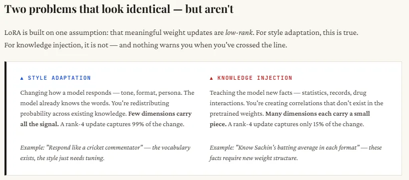
LoRA is widely used to fine-tune large models because it is efficient, but it tacitly assumes that all model updates are the same. In fact, they are not. If you’re singing a style well (like tone, form, or persona), changes are simple and focused on a few dimensions – which LoRA handles well with low-level updates. But if you try to teach the model new real-world information (like medical data or statistics), the information is spread over many places. A low level setting (like 8 levels) cannot capture everything, so the model may sound good but give incorrect or incomplete answers.
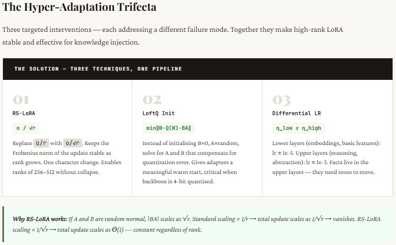
Trying to fix this by increasing the rate introduces another problem: instability. As the rate increases, the scaling used in standard LoRA causes the learning signal to weaken, making training ineffective. RS-LoRA solves this by slightly modifying the scaling formula (it changes from dividing by r dividing by √r), which stabilizes learning even at higher levels. This small change allows the model to better retain complex, high-level information without breaking training.
In the code snippet below, we show this failure in the first steps using NumPy – no training loops, no parameters. We simulate two types of weight updates, we directly measure how much information is weighted at each level, and we reveal the second failure: that increases the level unknowingly to compensate which causes a degradation of the scale that kills the learning signal completely. We then show the correction – the stable scaling of the RS-LoRA rate – and why one character change to a lower value (r → √r) is what makes the higher rate stable.

import numpy as np
import matplotlib.pyplot as plt
import matplotlib.gridspec as gridspec

np.random.seed(42)
In this setup, we simulate how fine tuning affects the weight matrix model by creating a simplified surface. We take a pre-trained weight matrix of size 64×64 and introduce two types of updates: low-level “stylistic” changes (like tone or formatting) and high-level “truth” changes (like detailed cricket stats). We then define two LoRA configurations — a small scale (r=4), which represents typical LoRA applications, and a large scale (r=32), which is more suitable for complex information capture as in RS-LoRA. This allows us to compare how well different standards can return these simulated updates and highlight where traditional LoRA struggles.
d, k = 64, 64 # weight matrix dimensions
r_low = 4 # LoRA rank -- small (standard choice)
r_high = 32 # LoRA rank -- large (RS-LoRA compatible)
print(f"Weight matrix shape : ({d} x {k})")
print(f"Low rank (standard): r = {r_low}")
print(f"High rank (RS-LoRA) : r = {r_high}")
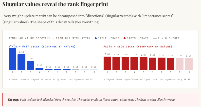
print(f"Max possible rank : {min(d, k)}")Here, we model two fundamentally different types of fine-tuning updates. The style review is deliberately structured as low-level: only a few singular values are large and the others decrease rapidly, meaning that most important information is concentrated in a few dimensions. This reflects real-world behavior where tone or formatting changes do not require extensive modification of the model.
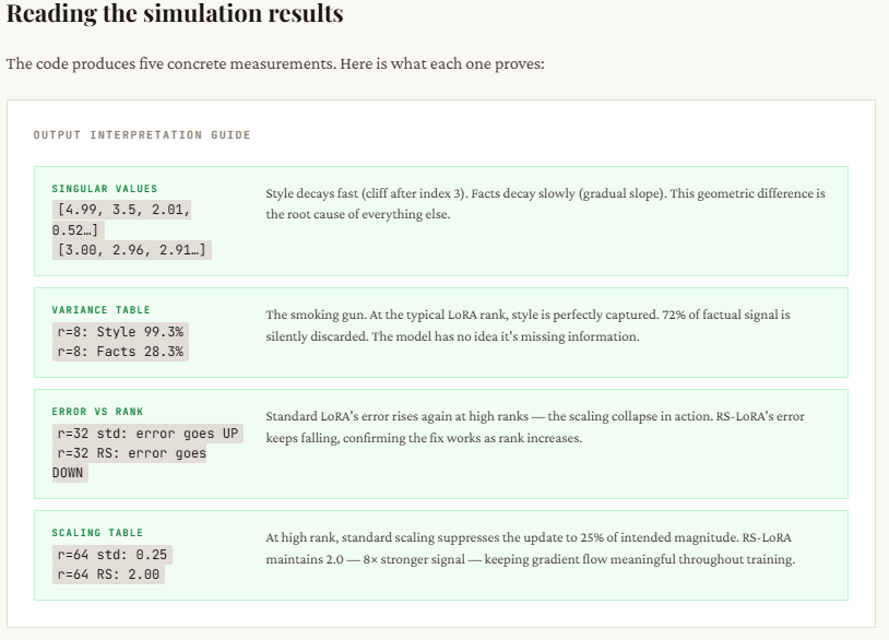
In contrast, the truth update has a high rate: singular values decrease slightly, indicating that many measurements provide useful information. This shows how factual information (such as statistics or domain data) is distributed throughout the model. The singular printed values make this clear – the stylistic updates show a large decrease after the first few values, while the true updates remain equally large across most measurements, proving that they cannot be easily compressed into lower estimates.
def make_low_rank_delta(d, k, true_rank, noise=0.01):
    """Simulates a style update -- low intrinsic rank."""
    U = np.random.randn(d, true_rank)
    S = np.linspace(5, 0.5, true_rank)   # fast-decaying singular values
    V = np.random.randn(k, true_rank)
    U, _ = np.linalg.qr(U)
    V, _ = np.linalg.qr(V)
    delta = (U[:, :true_rank] * S) @ V[:, :true_rank].T
    delta += noise * np.random.randn(d, k)
    return delta

def make_high_rank_delta(d, k, noise=0.01):
    """Simulates a fact/knowledge update -- high intrinsic rank."""
    U = np.random.randn(d, d)
    S = np.linspace(3, 0.5, min(d, k))   # slow-decaying -- many dimensions matter
    V = np.random.randn(k, k)
    U, _ = np.linalg.qr(U)
    V, _ = np.linalg.qr(V)
    delta = (U[:, :min(d,k)] * S) @ V[:, :min(d,k)].T
    delta += noise * np.random.randn(d, k)
    return delta

delta_style = make_low_rank_delta(d, k, true_rank=4)
delta_facts = make_high_rank_delta(d, k)

print("nStyle  update -- top 10 singular values:", np.linalg.svd(delta_style, compute_uv=False)[:10].round(2))
print("Facts  update -- top 10 singular values:", np.linalg.svd(delta_facts,  compute_uv=False)[:10].round(2))
print("nNotice: Style decays fast → low-rank. Facts decay slowly → high-rank.")
This section compares how standard LoRA and RS-LoRA can reconstruct real updates using different standards. Both methods first use SVD to find the best estimate of r-levels (ie, compress the update into r-levels), but they differ in how they measure the result: standard LoRA divides by r, while RS-LoRA divides by √r. The table shows the reconstruction error — lower means better.
The key takeaway is clear: for style updates, even small levels (like 4 or 8) work well because the information is inherently low-level, so the error decreases quickly. But with true reviews, the error is always high at low levels, which proves that important information is lost. Upscaling helps, but regular LoRA is unstable due to overscaling (the error is not always improving). RS-LoRA, with its √r scaling, handles high levels very well and reduces error gradually, making it better suited for capturing complex, high-dimensional information.
def lora_approx_standard(delta, r, alpha=16):
"""Approximate delta using rank-r LoRA with standard alpha/r scaling."""
U, S, Vt = np.linalg.svd(delta, full_matrices=False)
# Truncate to rank r
B = U[:, :r] * S[:r] # shape (d, r)
A = Vt[:r, :] # shape (r, k)
scaling = alpha / r
delta_approx = scaling * (B @ A)
error = np.linalg.norm(delta - delta_approx, 'fro') / np.linalg.norm(delta, 'fro')
return delta_approx, error
def lora_approx_rslora(delta, r, alpha=16):
"""Approximate delta using rank-r LoRA with RS-LoRA sqrt(r) scaling."""
U, S, Vt = np.linalg.svd(delta, full_matrices=False)
B = U[:, :r] * S[:r]
A = Vt[:r, :]
scaling = alpha / np.sqrt(r) # <-- the key change
delta_approx = scaling * (B @ A)
error = np.linalg.norm(delta - delta_approx, 'fro') / np.linalg.norm(delta, 'fro')
return delta_approx, error
ranks = [2, 4, 8, 16, 32, 48]
style_errors_standard, facts_errors_standard = [], []
style_errors_rslora, facts_errors_rslora = [], []
for r in ranks:
_, e = lora_approx_standard(delta_style, r); style_errors_standard.append(e)
_, e = lora_approx_standard(delta_facts, r); facts_errors_standard.append(e)
_, e = lora_approx_rslora(delta_style, r); style_errors_rslora.append(e)
_, e = lora_approx_rslora(delta_facts, r); facts_errors_rslora.append(e)
print("Rank | Style Err (std) | Facts Err (std) | Facts Err (RS-LoRA)")
print("-" * 60)
for i, r in enumerate(ranks):
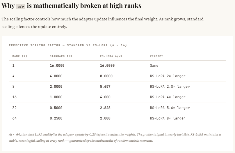
print(f" {r:2d} | {style_errors_standard[i]:.3f} | {facts_errors_standard[i]:.3f} | {facts_errors_rslora[i]:.3f}")This section explains why standard LoRA struggles at high levels. As the rate r increases, the standard LoRA scales the update by α / r, which decreases rapidly – you can see it drop from 16 (at r=1) to just 0.25 (at r=64). This means that even if you add more dimensions (trying to capture more information), the overall update becomes weaker and weaker, effectively suppressing the reading signal. The optimizer then compensates by pushing the levers harder, which often leads to instability or poor convergence.
RS-LoRA corrects this by changing the scaling to α / √r. Instead of decreasing dramatically, the scale decreases gradually – it remains strong enough even at high positions (eg, it is 2.0 at r=64). This keeps the size of the active update meaningful, allowing the model to actually benefit from high-level actions without killing the signal. In simple words: conventional LoRA adds capacity but kills its impact, while RS-LoRA preserves both.
alpha = 16
rs = np.arange(1, 65)
standard_scale = alpha / rs
rslora_scale   = alpha / np.sqrt(rs)

print("nRank | Standard Scale (alpha/r) | RS-LoRA Scale (alpha/sqrt(r))")
print("-" * 55)
for r in [1, 4, 8, 16, 32, 64]:
    print(f"  {r:2d} |         {alpha/r:.4f}          |         {alpha/np.sqrt(r):.4f}")

print("nStandard scaling vanishes as rank grows.")
print("RS-LoRA scaling stays meaningful at high ranks.")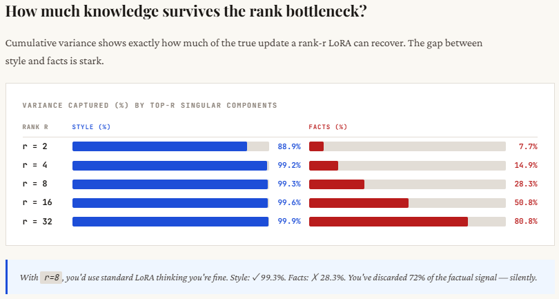
This section shows the main difference in how information is distributed between style and real updates. Stylistically, most of the important signal is concentrated in a few dimensions – you can see that by level 4, more than 99% of the information has been captured. This is why low-level methods like LoRA work best with tone, format, or personality changes. There is a clear “elbow” in the unique values — after a few parts, the others don’t matter so much.
In fact, it’s the opposite. Information is spread across multiple dimensions – even at level 8, you’re only capturing about 28% of the total signal, which means a lot of information is still missing. This is the problem of the “long tail”: the extra dimension gives something important. When LoRA is reduced to a low level, it cuts off this tail, resulting in incomplete or incorrect information. This is why a model may sound optimistic but get the facts wrong.
sv_style = np.linalg.svd(delta_style, compute_uv=False)
sv_facts  = np.linalg.svd(delta_facts,  compute_uv=False)

print("Cumulative variance captured by top-r components:n")
print(f"{'Rank':>5} | {'Style (%)':>10} | {'Facts (%)':>10}")
print("-" * 32)
total_style = np.sum(sv_style**2)
total_facts  = np.sum(sv_facts**2)
for r in [2, 4, 8, 16, 32]:
    cs = 100 * np.sum(sv_style[:r]**2) / total_style
    cf = 100 * np.sum(sv_facts[:r]**2)  / total_facts
    print(f"  {r:3d} | {cs:9.1f}% | {cf:9.1f}%")

print("nWith r=8, style is nearly fully captured.")
print("With r=8, facts are still poorly captured -- the tail matters!")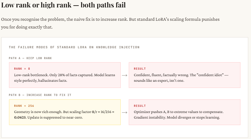
Check it out Full Codes here. Get 100s of ML/Data Science Colab Notebooks here. Also, feel free to follow us Twitter and don’t forget to join our 130k+ ML SubReddit and Subscribe to Our newspaper. Wait! are you on telegram? now you can join us on telegram too.
Need to work with us on developing your GitHub Repo OR Hug Face Page OR Product Release OR Webinar etc.? contact us

I am a Civil Engineering Graduate (2022) from Jamia Millia Islamia, New Delhi, and I am very interested in Data Science, especially Neural Networks and its application in various fields.


